Plot a dependent variable versus time
Usage
plot_dvtime(
  data,
  dv_var = "DV",
  time_var = "TIME",
  ntime_var = "NTIME",
  col_var = NULL,
  id_var = NULL,
  dose_var = "DOSE",
  loq = NULL,
  loq_method = 0,
  cent = c("mean", "mean_sdl", "mean_sdl_upper", "median", "median_iqr", "none"),
  dosenorm = FALSE,
  ref = NULL,
  log_y = FALSE,
  show_caption = TRUE,
  theme = NULL
)
Arguments
- data
Input dataset.
- dv_var
Column containing the dependent variable. Accepts bare names or strings. Default is
DV.- time_var
Column containing the actual time variable. Accepts bare names or strings. Default is
TIME.- ntime_var
Column containing the nominal time variable. Accepts bare names or strings. Default is
NTIME.- col_var
Column to map to the color aesthetic. Accepts bare names or strings. Default is
NULL.- id_var
Column to group observations for spaghetti lines. Accepts bare names or strings. Default is
NULL(no spaghetti lines). Specifying a column (e.g.,id_var = ID) enables spaghetti lines connecting observations within each level of the variable.- dose_var
Column to use in dosenormalization when
dosenorm= TRUE. Accepts bare names or strings. Default isDOSE.- loq
Numeric value of the lower limit of quantification (LLOQ) for the assay. Must be coercible to a numeric if specified. Can be
NULLif variableLLOQis present indataSpecifying this argument implies thatDVis missing indatawhere < LLOQ.- loq_method
Method for handling data below the lower limit of quantification (BLQ) in the plot.
Options are:
+ No handling: `0` or `"none"`, Plot input dataset `DV` vs `TIME` as is. (default) + Impute Post-dose: `1` or `"postdose"`, Impute all BLQ data at `TIME` <= 0 to 0 and all BLQ data at `TIME` > 0 to 1/2 x `loq`. Useful for plotting concentration-time data with some data BLQ on the linear scale + Impute All: `2` or `"all"`,Impute all BLQ data to 1/2 x `loq`. Useful for plotting concentration-time data with some data BLQ on the log scale where 0 cannot be displayed- cent
Character string specifying the central tendency measure to plot.
Options are:
Mean only:
"mean"(default)Mean +/- Standard Deviation (upper and lower error bar):
"mean_sdl"Mean + Standard Deviation (upper error bar only):
"mean_sdl_upper"Median only:
"median"Median +/- Interquartile Range:
median_iqrNone:
"none"
- dosenorm
logical indicating if observed data points should be dose normalized. Default is
FALSE, Requires variable specified indose_varto be present indata- ref
Numeric y-intercept for a horizontal reference line, or
NULLfor no reference line. For example,ref = 0draws a baseline reference for change-from-baseline data.- log_y
Logical indicator for log10 transformation of the y-axis. Also controls whether the caption reports arithmetic or geometric mean when
show_caption = TRUE.- show_caption
Logical indicating if a caption should be shown describing the data plotted
- theme
Theme object created by
plot_dvtime_theme(). Defaults can be viewed by runningplot_dvtime_theme()with no arguments. Default error bar width is 2.5% of maximumNTIME.
See also
Other exploratory analysis:
plot_dvconc(),
plot_dvconc_theme(),
plot_dvtime_theme()
Examples
data_sad_pk <- dplyr::filter(data_sad, CMT %in% c(1,2))
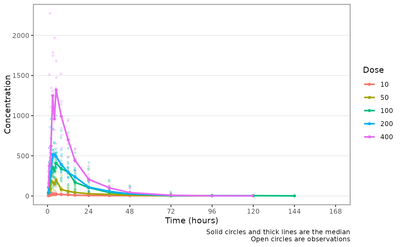
data <- dplyr::mutate(data_sad_pk, Dose = var_addn(DOSE, ID, sep = "mg"))
plot_dvtime(data, dv_var = ODV, cent = "median", col_var = Dose)
#> Warning: Removed 169 rows containing non-finite outside the scale range
#> (`stat_summary()`).
#> Warning: Removed 169 rows containing non-finite outside the scale range
#> (`stat_summary()`).
#> Warning: Removed 169 rows containing missing values or values outside the scale range
#> (`geom_point()`).