VPC Plot Aesthetics • pmxhelpr

This vignette will review the functionality for updating aesthetic elements of VPC plots generated using vpc() with the new_vpc_theme() function from the vpc package.

plot_legend() is a helper plotting function that creates a legend for plots generated using vpc(). These legends can then be merged with the VPC plot into a single plot object using the patchwork package.

Let’s get started. First, we will load the required packages.

options(scipen = 999, rmarkdown.html_vignette.check_title = FALSE)
library(pmxhelpr)
library(dplyr, warn.conflicts =  FALSE)
library(ggplot2, warn.conflicts =  FALSE)
library(vpc, warn.conflicts =  FALSE)
library(mrgsolve, warn.conflicts =  FALSE)
library(withr, warn.conflicts =  FALSE)
library(patchwork, warn.conflicts = FALSE)

Next, let’s load use the internal data and model objects from pmxhelpr and df_mrgsim_replicate to run the simulation.

data <- data_sad
model <- model_mread_load("model")
#> Building model_cpp ... done.

simout <- df_mrgsim_replicate(data = data, model = model,replicates = 100, 
                     dv_var = "ODV",
                     time_vars = c(TIME = "TIME", NTIME = "NTIME"),
                     output_vars = c(PRED = "PRED", IPRED = "IPRED", DV = "DV"),
                     num_vars = c("CMT", "BLQ", "LLOQ", "EVID", "MDV", "DOSE", "FOOD"),
                     char_vars = c("PART"),
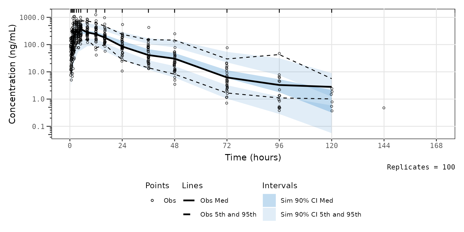
                     obsonly = TRUE)

Now let’s plot all data together in a prediction-corrected VPC (pcVPC). There is only single dose administration in this dataset, thus we are able to pool across doses and food conditions with prediction-correction. We will set min_bin_count = 5 to avoid the simulated intervals extending to the final timepoint with only a single observation.

vpc_pc <- plot_vpc_exactbins(
  sim = simout,
  xlab = "Time (hours)",
  ylab = "Concentration (ng/mL)",
  pcvpc = TRUE,
  min_bin_count = 5
) +
  scale_y_log10(guide = "axis_logticks")
#> Joining with `by = join_by(NTIME, CMT)`
#> Joining with `by = join_by(NTIME, CMT)`

vpc_pc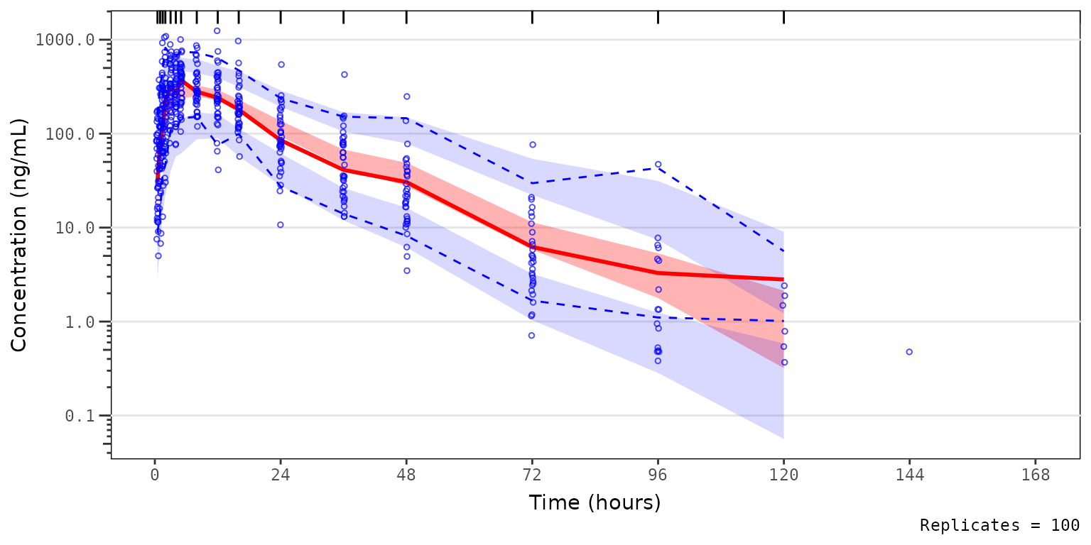

Plot Elements

Default Elements

The default elements shown in the plot are inherited from vpc(). The shown argument can be provided to plot_vpc_exactbins() and passed on to the show argument of vpc().

The default is as follows:

shown_list <- list(obs_dv = TRUE, obs_ci = TRUE,
                   pi = FALSE, pi_as_area = FALSE, pi_ci = TRUE,
                   obs_median = TRUE, sim_median =FALSE, sim_median_ci = TRUE)

The components of the list correspond to the following vpc plot elements:

Observed points: obs_dv
Observed quantiles: obs_ci
Simulated inter-quantile range: pi
Simulated inter-quantile area: pi_as_area
Simulated Quantile CI: pi_ci
Observed Median: obs_median
Simulated Median: sim_median
Simulated Median CI: sim_median_ci

One or more elements to be updated from the defaults above can be passed as a list to the argument shown. Any elements not specified in shown will inherit the defaults.

Adjusting Elements

For example, we may want to visualize the 90% prediction interval (i.e., 5th to 95th percentiles) derived from the simulation, rather than the confidence intervals of the 5th and 95th percentiles independently. In this case, we want to also see how close the simulated median falls relative to the observed median.

Let’s see how this can be down using shown!


vpc_pc_pi <- plot_vpc_exactbins(
  sim = simout, 
  time_vars = c(TIME = "TIME", NTIME = "NTIME"),
  output_vars = c(PRED = "PRED", IPRED = "IPRED", SIMDV = "SIMDV", OBSDV = "OBSDV"),
  xlab = "Time (hours)",
  ylab = "Concentration (ng/mL)",
  pcvpc = TRUE,
  min_bin_count = 5,
  shown = list(obs_ci = FALSE, pi_ci = FALSE, sim_median_ci = FALSE, sim_median = TRUE, pi_as_area = TRUE)
) +
  scale_y_log10(guide = "axis_logticks")
#> Joining with `by = join_by(NTIME, CMT)`
#> Joining with `by = join_by(NTIME, CMT)`

vpc_pc_pi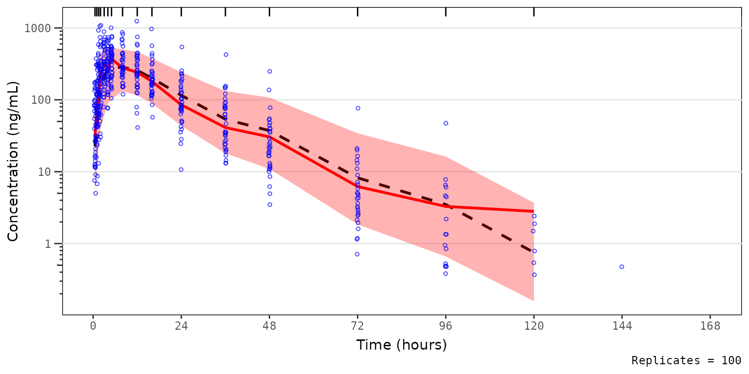

Now, let’s say we want to remove the observed data points from the plot above to better visualize the observed quantile lines relative to their corresponding simulated confidence intervals. We can do this as follows.


vpc_pc_noobs <- plot_vpc_exactbins(
  sim = simout, 
  time_vars = c(TIME = "TIME", NTIME = "NTIME"),
  output_vars = c(PRED = "PRED", IPRED = "IPRED", SIMDV = "SIMDV", OBSDV = "OBSDV"),
  xlab = "Time (hours)",
  ylab = "Concentration (ng/mL)",
  pcvpc = TRUE,
  min_bin_count = 5,
  shown = list(obs_dv = FALSE)
) +
  scale_y_log10(guide = "axis_logticks")
#> Joining with `by = join_by(NTIME, CMT)`
#> Joining with `by = join_by(NTIME, CMT)`

vpc_pc_noobs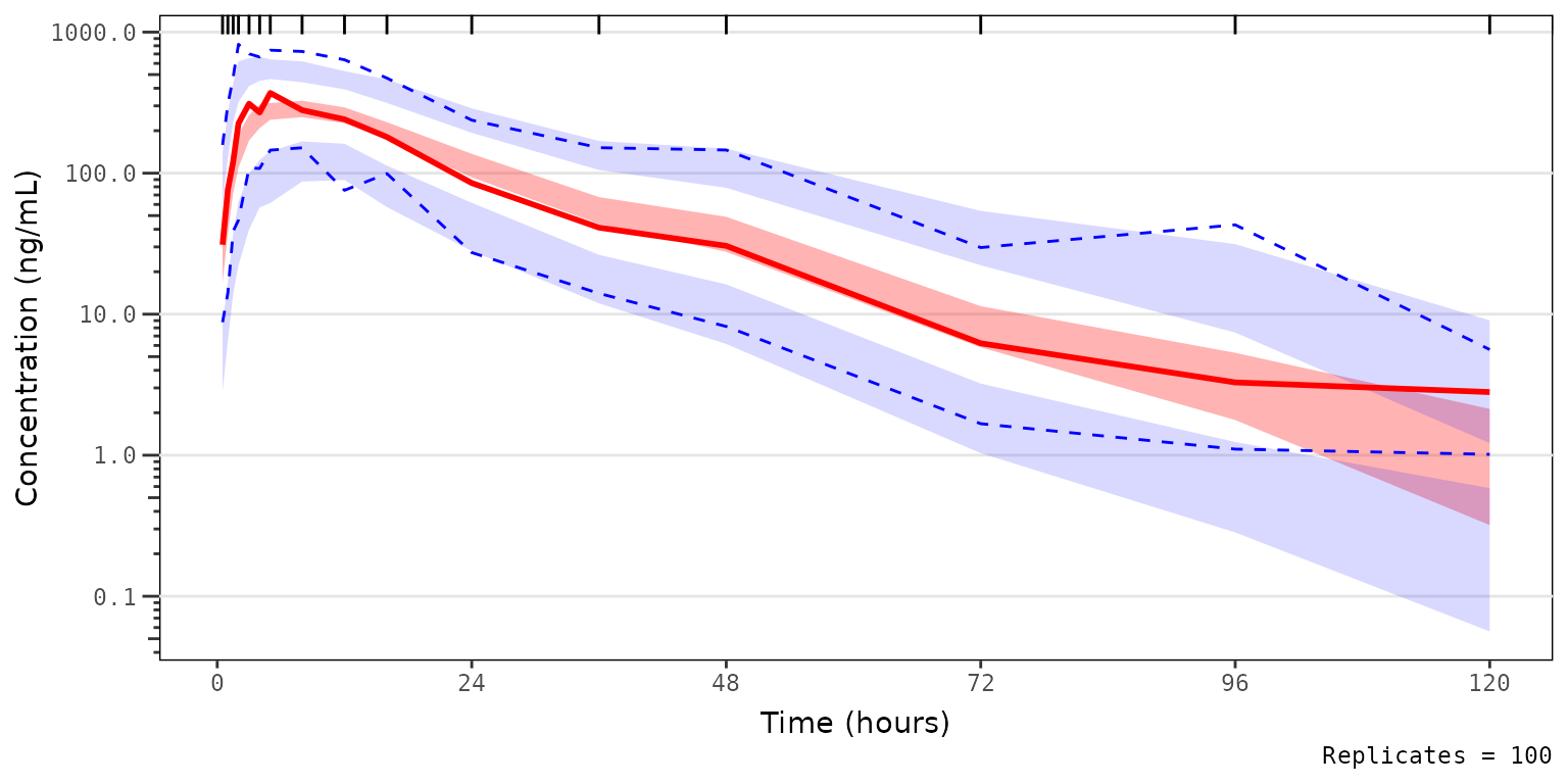

We could also take this one step further and only look at the median and the simulated confidence interval of the median, to closely interrogate central tendency. This is common for VPC strata which have few observations, leading to inadequate sample size to discriminate between the confidence intervals of the median and the extremes. This is common scenario when evaluating VPC plots stratified by individual study arms in early phase trials.


vpc_pc_noobs_medonly <- plot_vpc_exactbins(
  sim = simout, 
  time_vars = c(TIME = "TIME", NTIME = "NTIME"),
  output_vars = c(PRED = "PRED", IPRED = "IPRED", SIMDV = "SIMDV", OBSDV = "OBSDV"),
  xlab = "Time (hours)",
  ylab = "Concentration (ng/mL)",
  pcvpc = TRUE,
  min_bin_count = 5,
  shown = list(obs_dv = FALSE, obs_ci = FALSE, pi_ci = FALSE)
) +
  scale_y_log10(guide = "axis_logticks")
#> Joining with `by = join_by(NTIME, CMT)`
#> Joining with `by = join_by(NTIME, CMT)`

vpc_pc_noobs_medonly

Plot Aesthetics

Default Aesthetics

Similarly, the default aesthetics for vpc plots in pmxhelpr use the classical red-blue-green brewer color schema. The defaults for pmxhelpr can be visualized by specifying the pmxhlepr_vpc_theme() function with no arguments.

pmxhelpr_theme_list <- pmxhelpr_vpc_theme()
print(pmxhelpr_theme_list)
#> $obs_color
#> [1] "#0000FF"
#> 
#> $obs_size
#> [1] 1
#> 
#> $obs_median_color
#> [1] "#FF0000"
#> 
#> $obs_median_linetype
#> [1] "solid"
#> 
#> $obs_median_size
#> [1] 1
#> 
#> $obs_alpha
#> [1] 0.7
#> 
#> $obs_shape
#> [1] 1
#> 
#> $obs_ci_color
#> [1] "#0000FF"
#> 
#> $obs_ci_linetype
#> [1] "dashed"
#> 
#> $obs_ci_fill
#> [1] "#80808033"
#> 
#> $obs_ci_size
#> [1] 0.5
#> 
#> $sim_pi_fill
#> [1] "#0000FF"
#> 
#> $sim_pi_alpha
#> [1] 0.15
#> 
#> $sim_pi_color
#> [1] "#000000"
#> 
#> $sim_pi_linetype
#> [1] "dotted"
#> 
#> $sim_pi_size
#> [1] 1
#> 
#> $sim_median_fill
#> [1] "#FF0000"
#> 
#> $sim_median_alpha
#> [1] 0.3
#> 
#> $sim_median_color
#> [1] "#000000"
#> 
#> $sim_median_linetype
#> [1] "dashed"
#> 
#> $sim_median_size
#> [1] 1
#> 
#> $bin_separators_color
#> [1] "#000000"
#> 
#> $loq_color
#> [1] "#990000"
#> 
#> attr(,"class")
#> [1] "vpc_theme"

We can compare to the corresponding aesthetics from the vpc package, which can be viewed by running new_vpc_theme() with no arguments.

vpc_theme_list <- new_vpc_theme()
print(vpc_theme_list)
#> $obs_color
#> [1] "#000000"
#> 
#> $obs_size
#> [1] 1
#> 
#> $obs_median_color
#> [1] "#000000"
#> 
#> $obs_median_linetype
#> [1] "solid"
#> 
#> $obs_median_size
#> [1] 1
#> 
#> $obs_alpha
#> [1] 0.7
#> 
#> $obs_shape
#> [1] 1
#> 
#> $obs_ci_color
#> [1] "#000000"
#> 
#> $obs_ci_linetype
#> [1] "dashed"
#> 
#> $obs_ci_fill
#> [1] "#80808033"
#> 
#> $obs_ci_size
#> [1] 0.5
#> 
#> $sim_pi_fill
#> [1] "#3388cc"
#> 
#> $sim_pi_alpha
#> [1] 0.15
#> 
#> $sim_pi_color
#> [1] "#000000"
#> 
#> $sim_pi_linetype
#> [1] "dotted"
#> 
#> $sim_pi_size
#> [1] 1
#> 
#> $sim_median_fill
#> [1] "#3388cc"
#> 
#> $sim_median_alpha
#> [1] 0.3
#> 
#> $sim_median_color
#> [1] "#000000"
#> 
#> $sim_median_linetype
#> [1] "dashed"
#> 
#> $sim_median_size
#> [1] 1
#> 
#> $bin_separators_color
#> [1] "#000000"
#> 
#> $loq_color
#> [1] "#990000"
#> 
#> attr(,"class")
#> [1] "vpc_theme"

Adjusting Aesthetics

Now, suppose we want to change the default aesthetics of the VPC plot, without changing what is being shown. This can be accomplished by passing a named list of elements to update to the function pmxhelpr_vpc_theme(). The named list object generated from this function can then be passed to the theme argument in vpc_plot_exactbins, which is also an alias for the vpc_theme argument in vpc().

Let’s say we prefer a the blue-grey color scheme native to the vpc package! We can reproduce this by passing vpc::new_vpc_theme():

to the update argument of pmxhelpr_vpc_theme()

vpc_pc_vpctheme <- plot_vpc_exactbins(
  sim = simout, 
  time_vars = c(TIME = "TIME", NTIME = "NTIME"),
  output_vars = c(PRED = "PRED", IPRED = "IPRED", SIMDV = "SIMDV", OBSDV = "OBSDV"),
  xlab = "Time (hours)",
  ylab = "Concentration (ng/mL)",
  pcvpc = TRUE,
  theme = pmxhelpr_vpc_theme(update = vpc::new_vpc_theme()),
  min_bin_count = 5
) +
  scale_y_log10(guide = "axis_logticks")
#> Joining with `by = join_by(NTIME, CMT)`
#> Joining with `by = join_by(NTIME, CMT)`

vpc_pc_vpctheme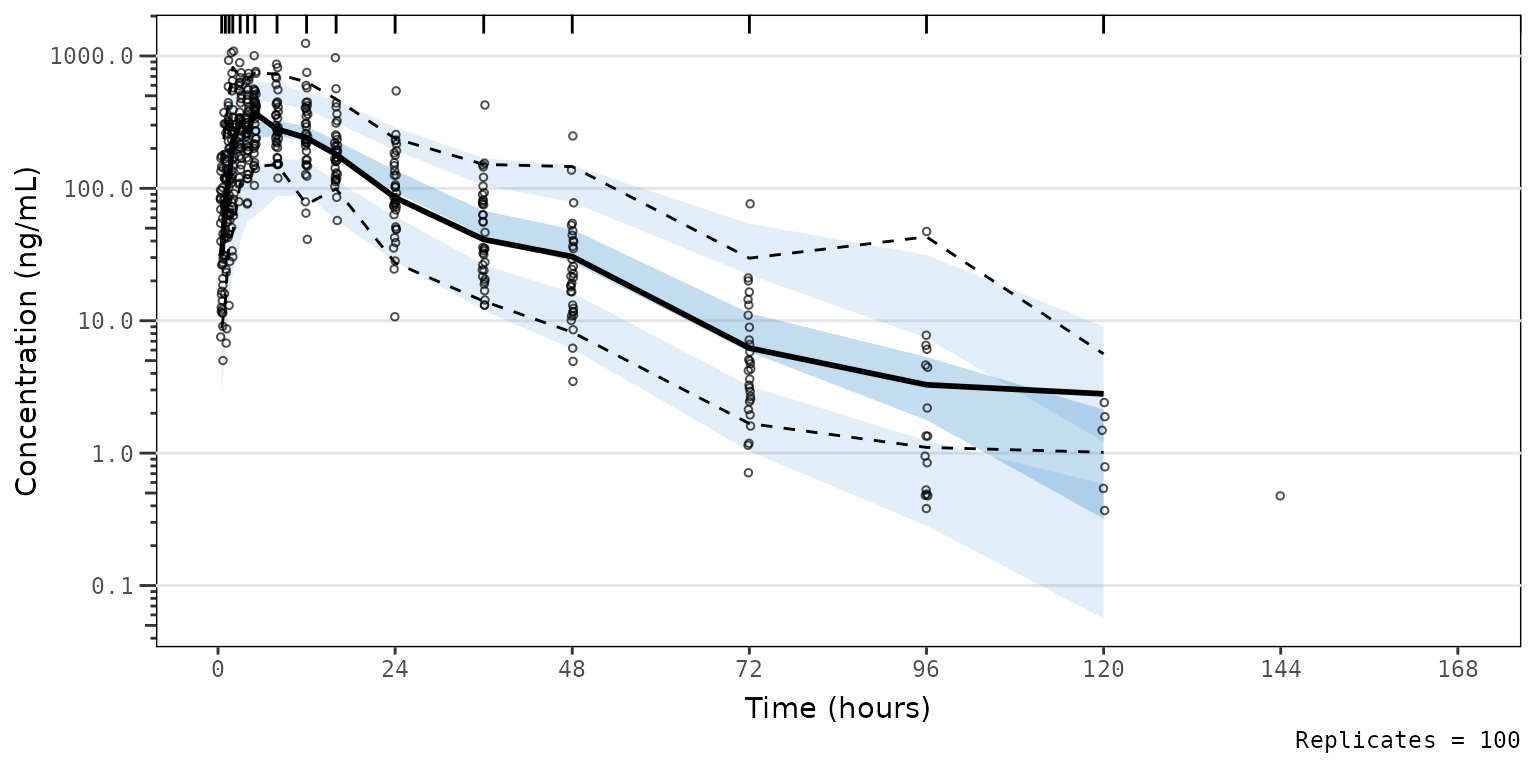

2) to the theme argument of plot_vpc_exactbins.

vpc_pc_vpctheme2 <- plot_vpc_exactbins(
  sim = simout, 
  time_vars = c(TIME = "TIME", NTIME = "NTIME"),
  output_vars = c(PRED = "PRED", IPRED = "IPRED", SIMDV = "SIMDV", OBSDV = "OBSDV"),
  xlab = "Time (hours)",
  ylab = "Concentration (ng/mL)",
  pcvpc = TRUE,
  theme = vpc::new_vpc_theme(),
  min_bin_count = 5
) +
  scale_y_log10(guide = "axis_logticks")
#> Joining with `by = join_by(NTIME, CMT)`
#> Joining with `by = join_by(NTIME, CMT)`

vpc_pc_vpctheme2

Adding Layers

Let’s say we would like to visualize the major x-axis grid lines to help locate data corresponding to each sampling timepoint with our plot using the vpc package aesthetic defaults. Conveniently, plot_vpc_exactbins returns a ggplot2 plot object, which we can modify by adding layers just like like any other ggplot2 object.

vpc_pc_vpctheme_xgrid <- plot_vpc_exactbins(
  sim = simout, 
  time_vars = c(TIME = "TIME", NTIME = "NTIME"),
  xlab = "Time (hours)",
  ylab = "Concentration (ng/mL)",
  pcvpc = TRUE,
  min_bin_count = 5,
  theme = vpc::new_vpc_theme()
) + 
  scale_y_log10(guide = "axis_logticks") + 
  theme(panel.grid.major.x = element_line())
#> Joining with `by = join_by(NTIME, CMT)`
#> Joining with `by = join_by(NTIME, CMT)`

vpc_pc_vpctheme_xgrid

VPC Plot Legends

Defaults Legend

Okay, now we have gotten the plot aesthetics where we want them; however, there is one other element we may like to include in the figure to make it more easily interpreted in isolation - a legend.

pmxhelpr provides a useful helper function for this purpose, plot_legend(). To obtain a legend for a plot using default aesthetics, simply run plot_legend() without any arguments specified.

vpc_pc_legend <- plot_legend()
vpc_pc_legend

Now we have a ggplot object legend for our first plot!

To generate one for our second plot with updated aesthetics to match the vpc package defaults, let’s pass the named list output from vpc::new_vpc_theme() to the update argument.

vpc_pc_new_legend <- plot_legend(update = vpc::new_vpc_theme())
vpc_pc_new_legend

Okay, now that we have our legend plot objects, let’s combine them with the VPC plot objects into a single plot object with the patchwork package.

vpc_pc_wleg <- vpc_pc + vpc_pc_legend + plot_layout(heights = c(2.5,1))
vpc_pc_wleg

vpc_pc_new_wleg <- vpc_pc_vpctheme_xgrid + vpc_pc_new_legend + plot_layout(heights = c(2.5,1))
vpc_pc_new_wleg