This vignette will review the limitations of the vpc()
function in the vpc package for datasets containing an
exact binning variable. This was the motivating reason for development
of plot_vpc_exactbins().
The vpcpackage offers a lot of great functionality to
generate VPC plots including, but certainly not limited to:
- data processing and visualization steps combined in one function
- built-in options for automatic binning for datasets without a binned time variable
- built-in option for prediction-correction
- built-in option for censoring at the lower limit of quantification (LLOQ)
However, although vpc() contains many great options to
automatically identify bins in the data, it is not optimized to leverage
input datasets with variable a variable representing exact bin times
(e.g., nominal, or protocol-specified, times).
First, we will load the required packages.
options(scipen = 999, rmarkdown.html_vignette.check_title = FALSE)
library(pmxhelpr)
library(dplyr, warn.conflicts =  FALSE)
library(ggplot2, warn.conflicts =  FALSE)
library(vpc, warn.conflicts =  FALSE)
library(mrgsolve, warn.conflicts =  FALSE)
library(withr, warn.conflicts =  FALSE)
Analysis Dataset
Next let’s explore the input dataset, data_sad. This
dataset was generated via simulation from model, an
mrgsolve model internal to the pmxhelpr package.
We can take a quick look at the dataset using glimpse()
from the dplyr package. Documentation for the dataset can also be viewed
using the R help functionality, just as one would for a function, with
?data_sad()
glimpse(data_sad)
#> Rows: 720
#> Columns: 23
#> $ LINE    <dbl> 1, 2, 3, 4, 5, 6, 7, 8, 9, 10, 11, 12, 13, 14, 15, 16, 17, 18,…
#> $ ID      <dbl> 1, 1, 1, 1, 1, 1, 1, 1, 1, 1, 1, 1, 1, 1, 1, 1, 1, 1, 1, 1, 2,…
#> $ TIME    <dbl> 0.00, 0.00, 0.48, 0.81, 1.49, 2.11, 3.05, 4.14, 5.14, 7.81, 12…
#> $ NTIME   <dbl> 0.0, 0.0, 0.5, 1.0, 1.5, 2.0, 3.0, 4.0, 5.0, 8.0, 12.0, 16.0, …
#> $ NDAY    <dbl> 1, 1, 1, 1, 1, 1, 1, 1, 1, 1, 1, 1, 2, 2, 3, 4, 5, 6, 7, 8, 1,…
#> $ DOSE    <dbl> 10, 10, 10, 10, 10, 10, 10, 10, 10, 10, 10, 10, 10, 10, 10, 10…
#> $ AMT     <dbl> NA, 10, NA, NA, NA, NA, NA, NA, NA, NA, NA, NA, NA, NA, NA, NA…
#> $ EVID    <dbl> 0, 1, 0, 0, 0, 0, 0, 0, 0, 0, 0, 0, 0, 0, 0, 0, 0, 0, 0, 0, 0,…
#> $ ODV     <dbl> NA, NA, NA, 2.02, 4.02, 3.50, 7.18, 9.31, 12.46, 13.43, 12.11,…
#> $ LDV     <dbl> NA, NA, NA, 0.7031, 1.3913, 1.2528, 1.9713, 2.2311, 2.5225, 2.…
#> $ CMT     <dbl> 2, 1, 2, 2, 2, 2, 2, 2, 2, 2, 2, 2, 2, 2, 2, 2, 2, 2, 2, 2, 2,…
#> $ MDV     <dbl> 1, NA, 1, 0, 0, 0, 0, 0, 0, 0, 0, 0, 0, 0, 1, 1, 1, 1, 1, 1, 1…
#> $ BLQ     <dbl> -1, NA, 1, 0, 0, 0, 0, 0, 0, 0, 0, 0, 0, 0, 1, 1, 1, 1, 1, 1, …
#> $ LLOQ    <dbl> 1, NA, 1, 1, 1, 1, 1, 1, 1, 1, 1, 1, 1, 1, 1, 1, 1, 1, 1, 1, 1…
#> $ FOOD    <dbl> 0, 0, 0, 0, 0, 0, 0, 0, 0, 0, 0, 0, 0, 0, 0, 0, 0, 0, 0, 0, 0,…
#> $ SEXF    <dbl> 1, 1, 1, 1, 1, 1, 1, 1, 1, 1, 1, 1, 1, 1, 1, 1, 1, 1, 1, 1, 1,…
#> $ RACE    <dbl> 2, 2, 2, 2, 2, 2, 2, 2, 2, 2, 2, 2, 2, 2, 2, 2, 2, 2, 2, 2, 1,…
#> $ AGEBL   <int> 25, 25, 25, 25, 25, 25, 25, 25, 25, 25, 25, 25, 25, 25, 25, 25…
#> $ WTBL    <dbl> 82.1, 82.1, 82.1, 82.1, 82.1, 82.1, 82.1, 82.1, 82.1, 82.1, 82…
#> $ SCRBL   <dbl> 0.87, 0.87, 0.87, 0.87, 0.87, 0.87, 0.87, 0.87, 0.87, 0.87, 0.…
#> $ CRCLBL  <dbl> 128, 128, 128, 128, 128, 128, 128, 128, 128, 128, 128, 128, 12…
#> $ USUBJID <chr> "STUDYNUM-SITENUM-1", "STUDYNUM-SITENUM-1", "STUDYNUM-SITENUM-…
#> $ PART    <chr> "Part 1-SAD", "Part 1-SAD", "Part 1-SAD", "Part 1-SAD", "Part …
This dataset is formatted for modeling. It contains NONMEM reserved variables (e.g., ID, TIME, AMT, EVID, MDV), as well as, dependent variables of drug concentration in original units (ODV) and natural logarithm transformed units (LDV). In addition to the numeric variables, there are two character variables: USUBJID and PART.
PART specifies the two study cohorts:
- Single Ascending Dose (SAD)
- Food Effect (FE).
unique(data_sad$PART)
#> [1] "Part 1-SAD" "Part 2-FE"
This dataset also contains an exact binning variable:
- Nominal Time (NTIME).
This variable represents the nominal time of sample collection relative to first dose per study protocol whereas Actual Time (TIME) represents the actual time the sample was collected.
PK Model
Luckily for us, someone has already fit a PK model to these data!
Let’s load model by calling model_mread_load()
and take a look at it with the see() function from the
mrgsolve package.
model <- model_mread_load("model")
#> Building model_cpp ... done.
see(model)
#>
#> Model file:  model.cpp
#> $PARAM
#> TVCL = 20
#> TVVC = 35.7
#> TVKA = 0.3
#> TVQ = 25
#> TVVP = 150
#> DOSE_F1 = 0.33
#>
#> WT_CL = 0.75
#> WT_VC = 1.00
#> WT_Q = 0.75
#> WT_VP = 1.00
#> FOOD_KA = -0.5
#> FOOD_F1 = 1.33
#>
#> WT = 70
#> DOSE = 100
#> FOOD = 0
#>
#> $CMT GUT CENT PERIPH TRANS1 TRANS2
#>
#> $MAIN
#> double CL = TVCL*pow(WT/70,WT_CL)*exp(ETA_CL);
#> double VC  = TVVC*pow(WT/70, WT_VC)*exp(ETA_VC);
#> double Q = TVCL*pow(WT/70,WT_Q)*exp(ETA_Q);
#> double VP  = TVVP*pow(WT/70, WT_VP)*exp(ETA_VP);
#> double KA = TVKA*(1+FOOD_KA*FOOD)*exp(ETA_KA);
#> double F1 = 1*(1+FOOD_F1*FOOD)*pow(DOSE/100,DOSE_F1);
#>
#> F_GUT = F1;
#>
#> $ODE
#> dxdt_GUT = -KA*GUT;
#> dxdt_CENT = KA*TRANS1 - (CL/VC)*CENT + (Q/VP)*PERIPH - (Q/VC)*CENT;
#> dxdt_PERIPH = (Q/VC)*CENT - (Q/VP)*PERIPH;
#> dxdt_TRANS1 = KA*GUT - KA*TRANS1;
#> dxdt_TRANS2 = KA*TRANS1 - KA*TRANS2;
#>
#> $OMEGA @labels ETA_CL ETA_VC ETA_KA ETA_Q ETA_VP
#> 0.075 0.1 0.2 0 0
#>
#> $SIGMA @labels PROP
#> 0.09
#>
#> $TABLE
#> capture IPRED = CENT/(VC/1000);
#> capture DV = IPRED*(1+PROP);
#> capture Y = DV;
Unluckily for us, no one has validated this PK model! Therefore, we need to generate some Visual Predictive Checks (VPCs).
VPC Plot Workflow
Running the simulation
We will use df_mrgsim_replicate() to run the simulation
for the VPC. df_mrgsim_replicate() is a wrapper function
for mrgsim_df(), which uses lapply() to
iterate the simulation over integers from 1 to the value passed to the
argument replicates.
We can pass data_sad and model from the
previous steps to the data and model
arguments, respectively, and run the simulation for 100
replicates. The names of actual and nominal time variables
in data_sad match the default arguments; however, our
dependent variable is named "ODV", which must be specified
in the dv_var argument, since it differs from the default
("DV").
We would like to recover the numerical variables "DOSE"
and "FOOD" and the character variable "PART"
from the input dataset, as we may need these study conditions to
stratify our VPC plots. We will request "BLQ" and
"LLOQ" for potential assessment of impact of censoring in
the VPCs, as well as, the NONMEM reserved variables "CMT",
"EVID", and "MDV". Finally, we will add the
argument obsonly = TRUE, which is passed to
mrgsim(), to remove dose records from the simulation output
and reduce file size.
simout <- df_mrgsim_replicate(data = data_sad,
                     model = model,
                     replicates = 100,
                     dv_var = "ODV",
                     time_vars = c(TIME = "TIME", NTIME = "NTIME"),
                     output_vars = c(PRED = "PRED", IPRED = "IPRED", DV = "DV"),
                     num_vars = c("CMT", "BLQ", "LLOQ", "EVID", "MDV", "DOSE", "FOOD"),
                     char_vars = c("PART"),
                     obsonly = TRUE)

glimpse(simout)
#> Rows: 68,400
#> Columns: 22
#> $ ID     <dbl> 1, 1, 1, 1, 1, 1, 1, 1, 1, 1, 1, 1, 1, 1, 1, 1, 1, 1, 1, 2, 2, …
#> $ TIME   <dbl> 0.00, 0.48, 0.81, 1.49, 2.11, 3.05, 4.14, 5.14, 7.81, 12.08, 16…
#> $ NTIME  <dbl> 0.0, 0.5, 1.0, 1.5, 2.0, 3.0, 4.0, 5.0, 8.0, 12.0, 16.0, 24.0, …
#> $ PRED   <dbl> 0.0000000000, 1.0373644222, 2.4699025938, 5.8692716205, 8.67222…
#> $ IPRED  <dbl> 0.00000000000, 0.23991271053, 0.58097762508, 1.44344928000, 2.2…
#> $ SIMDV  <dbl> 0.0000000000, 0.2070745747, 0.6769646573, 1.8613297145, 1.74160…
#> $ OBSDV  <dbl> NA, NA, 2.02, 4.02, 3.50, 7.18, 9.31, 12.46, 13.43, 12.11, 11.0…
#> $ EVID   <dbl> 0, 0, 0, 0, 0, 0, 0, 0, 0, 0, 0, 0, 0, 0, 0, 0, 0, 0, 0, 0, 0, …
#> $ CMT    <dbl> 2, 2, 2, 2, 2, 2, 2, 2, 2, 2, 2, 2, 2, 2, 2, 2, 2, 2, 2, 2, 2, …
#> $ BLQ    <dbl> -1, 1, 0, 0, 0, 0, 0, 0, 0, 0, 0, 0, 0, 1, 1, 1, 1, 1, 1, -1, 0…
#> $ LLOQ   <dbl> 1, 1, 1, 1, 1, 1, 1, 1, 1, 1, 1, 1, 1, 1, 1, 1, 1, 1, 1, 1, 1, …
#> $ MDV    <dbl> 1, 1, 0, 0, 0, 0, 0, 0, 0, 0, 0, 0, 0, 1, 1, 1, 1, 1, 1, 1, 0, …
#> $ DOSE   <dbl> 10, 10, 10, 10, 10, 10, 10, 10, 10, 10, 10, 10, 10, 10, 10, 10,…
#> $ FOOD   <dbl> 0, 0, 0, 0, 0, 0, 0, 0, 0, 0, 0, 0, 0, 0, 0, 0, 0, 0, 0, 0, 0, …
#> $ GUT    <dbl> 0.00000000000000000, 4.34652773939926984, 4.13276198317304821, …
#> $ CENT   <dbl> 0.000000000000, 0.009786371098, 0.023698880423, 0.058880291437,…
#> $ PERIPH <dbl> 0.00000000000, 0.00080390625, 0.00337854545, 0.01621962833, 0.0…
#> $ TRANS1 <dbl> 0.0000000000000000, 0.3188382667608536, 0.5115783540267899, 0.8…
#> $ TRANS2 <dbl> 0.00000000000000, 0.01169414527583, 0.03166313774719, 0.0965661…
#> $ Y      <dbl> 0.0000000000, 0.2070745747, 0.6769646573, 1.8613297145, 1.74160…
#> $ PART   <chr> "Part 1-SAD", "Part 1-SAD", "Part 1-SAD", "Part 1-SAD", "Part 1…
#> $ SIM    <int> 1, 1, 1, 1, 1, 1, 1, 1, 1, 1, 1, 1, 1, 1, 1, 1, 1, 1, 1, 1, 1, …

max(simout$SIM)
#> [1] 100
The maximum value of our replicate count variable (default =
"SIM") indicates that the dataset has been replicated 100
times.
Glimpsing the output reveals the following model outputs:
-
PRED(population prediction) -
IPRED(individual prediction) -
SIMDV(simulated dependent variable) -
OBSDV(observed dependent variable).
VPC plots with the vpc package
Now that we have run the simulation, we can generate VPC plots using
vpc().The documentation for vpc() (https://vpc.ronkeizer.com/binning.html) describes the
following binning methods:
-
time: Divide bins equally over time (or whatever independent variable is used). Recommended only when there is no observable clustering in the independent variable. -
data: Divide bins equally over the amount of data ordered by independent variable. Recommended only when data are for nominal timepoints and all datapoints are available. -
density: Divide bins based on data-density, i.e. place the bin-separators at nadirs in the density function. An approximate number of bins can be specified, but it is not certain that the algorithm will strictly use the specified number. More info in?auto_bin(). -
jenks: Default and recommended method. Jenk’s natural breaks optimization, similar to K-means clustering. -
kmeans: K-means clustering. -
pretty,quantile,hclust,sd,bclust,fisher. Methods provided by theclassIntpackage, see the package help for more information.
We can visualize the bins assigned by the various binning approaches
in vpc() using by assigning the plot as an object , let’s
call it plot_object, and calling
plot_object$data.
Because we have multiple dose levels in the SAD portion of the study,
as well as, a food effect cohort, prediction-correction will be used to
plot all the data on a single plot using the argument
pred_corr = TRUE.
vpc_jenks <- vpc(
  sim = simout,
  obs = filter(simout, SIM == 1),
  bins = "jenks", #default
  n_bins = "auto",
  sim_cols = list(dv = "SIMDV", idv = "NTIME", pred = "PRED"),
  obs_cols = list(dv = "OBSDV", idv = "NTIME", pred = "PRED"),
  pred_corr = TRUE,
  pi = c(0.05, 0.95),
  ci = c(0.05, 0.95),
  show = list(obs_dv = TRUE),
  log_y = TRUE,
  xlab = "Time (hours)",
  ylab = "PRED-corrected Concentration (ng/mL)"
) +
  scale_x_continuous(breaks = seq(0,168,24))

vpc_jenks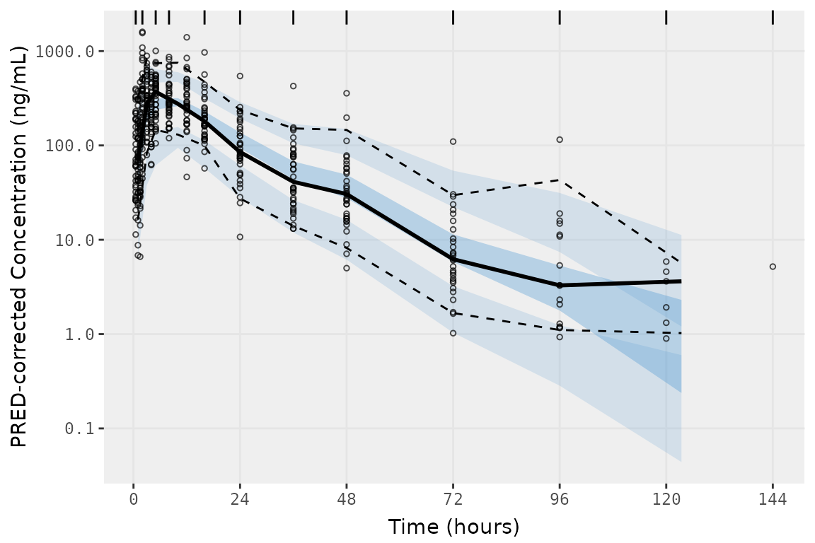
This plot looks pretty good! The default binning in
vpc::vpc() produce a very nice looking plot. However, all
of the binning methods internal to vpc() are designed to
determine binning intervals from the data. Currently, there is no method
to use exact bins contained in the data in place of bin
intervals determined from the data. The presence of exact bins in
the data is a common scenario in pharmacometrics, as Clinical Study
Protocols usually specific Study Days and times for collection.
We can use the df_nobsbin() function to calculate and
return a summary data.frame containing the unique exact bin times, count
of non-missing observations (EVID=0 & MDV=0), and count of missing
(EVID=0 & MDV=1) observations.
##Exact bins in the input data
df_nobsbin(data_sad, bin_var = "NTIME")
#> # A tibble: 19 × 4
#>    NTIME   CMT n_obs n_miss
#>    <dbl> <dbl> <int>  <int>
#>  1   0       2     0     36
#>  2   0.5     2    34      2
#>  3   1       2    36      0
#>  4   1.5     2    36      0
#>  5   2       2    36      0
#>  6   3       2    36      0
#>  7   4       2    36      0
#>  8   5       2    36      0
#>  9   8       2    36      0
#> 10  12       2    36      0
#> 11  16       2    36      0
#> 12  24       2    36      0
#> 13  36       2    36      0
#> 14  48       2    33      3
#> 15  72       2    29      7
#> 16  96       2    16     20
#> 17 120       2     6     30
#> 18 144       2     1     35
#> 19 168       2     0     36

##Bin midpoints and boundaries determined by vpc() using bins = "jenks"
distinct(select(vpc_jenks$data, bin_mid, bin_min, bin_max))
#> Adding missing grouping variables: `strat`
#> # A tibble: 11 × 4
#> # Groups:   strat [1]
#>    strat bin_mid bin_min bin_max
#>    <fct>   <dbl>   <dbl>   <dbl>
#>  1 1        1.01     0.5       2
#>  2 1        3        2         5
#>  3 1        5        5         8
#>  4 1       10        8        16
#>  5 1       16       16        24
#>  6 1       24       24        36
#>  7 1       36       36        48
#>  8 1       48       48        72
#>  9 1       72       72        96
#> 10 1       96       96       120
#> 11 1      123.     120       144
The bin_mid variable is wherevpc() will
plot the summary statistics calculated for the observed and simulated
data.
We can clearly see that the default bins = "jenks"
method does not reproduce the exact bins in the observed dataset,
even when passing nominal, rather than actual, time as the
independent variable (idv). How about the other
binning methods native to vpc()?
Let’s take a look at bins = "pretty" next.
vpc_pretty <- vpc(
  sim = simout,
  obs = filter(simout, SIM == 1),
  bins = "pretty",
  n_bins = "auto",
  sim_cols = list(dv = "SIMDV", idv = "NTIME", pred = "PRED"),
  obs_cols = list(dv = "OBSDV", idv = "NTIME", pred = "PRED"),
  pred_corr = TRUE,
  pi = c(0.05, 0.95),
  ci = c(0.05, 0.95),
  show = list(obs_dv = TRUE),
  log_y = TRUE,
  xlab = "Time (hours)",
  ylab = "PRED-corrected Concentration (ng/mL)"
) +
  scale_x_continuous(breaks = seq(0,168,24))

vpc_pretty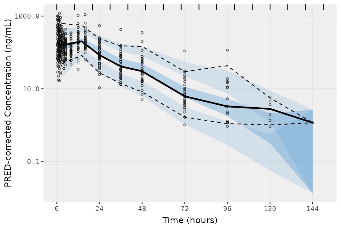
The vpc plot produced with bins = "pretty is
fairly pretty; however, again we can see that the binning is not true to
the exact bins in our dataset, especially at the earlier absorption
phase time-points, which are being largely binned together.
##Exact bins in the input data
df_nobsbin(data_sad, bin_var = "NTIME")
#> # A tibble: 19 × 4
#>    NTIME   CMT n_obs n_miss
#>    <dbl> <dbl> <int>  <int>
#>  1   0       2     0     36
#>  2   0.5     2    34      2
#>  3   1       2    36      0
#>  4   1.5     2    36      0
#>  5   2       2    36      0
#>  6   3       2    36      0
#>  7   4       2    36      0
#>  8   5       2    36      0
#>  9   8       2    36      0
#> 10  12       2    36      0
#> 11  16       2    36      0
#> 12  24       2    36      0
#> 13  36       2    36      0
#> 14  48       2    33      3
#> 15  72       2    29      7
#> 16  96       2    16     20
#> 17 120       2     6     30
#> 18 144       2     1     35
#> 19 168       2     0     36

##Bin midpoints and boundaries determined by vpc() using bins = "pretty"
distinct(select(vpc_pretty$data, bin_mid, bin_min, bin_max))
#> Adding missing grouping variables: `strat`
#> # A tibble: 9 × 4
#> # Groups:   strat [1]
#>   strat bin_mid bin_min bin_max
#>   <fct>   <dbl>   <dbl>   <dbl>
#> 1 1        3.14       0      10
#> 2 1       14         10      20
#> 3 1       24         20      30
#> 4 1       36         30      40
#> 5 1       48         40      50
#> 6 1       72         70      80
#> 7 1       96         90     100
#> 8 1      120        120     130
#> 9 1      144        140     150
The bins = "kmeans" option produces yet another
reasonable plot; however, like bins = "pretty", it groups
many of the absorption phase timepoints together and does not include
the last three sampling times with quantifiable observations in
simulated intervals.
vpc_kmeans <- vpc(
  sim = simout,
  obs = filter(simout, SIM == 1),
  bins = "kmeans",
  n_bins = "auto",
  sim_cols = list(dv = "SIMDV", idv = "NTIME", pred = "PRED"),
  obs_cols = list(dv = "OBSDV", idv = "NTIME", pred = "PRED"),
  pred_corr = TRUE,
  pi = c(0.05, 0.95),
  ci = c(0.05, 0.95),
  show = list(obs_dv = TRUE),
  log_y = TRUE,
  xlab = "Time (hours)",
  ylab = "PRED-corrected Concentration (ng/mL)"
) +
  scale_x_continuous(breaks = seq(0,168,24))

vpc_kmeans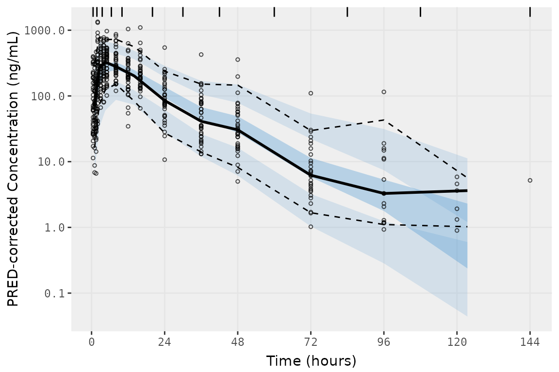
##Exact bins in the input data
df_nobsbin(data_sad, bin_var = "NTIME")
#> # A tibble: 19 × 4
#>    NTIME   CMT n_obs n_miss
#>    <dbl> <dbl> <int>  <int>
#>  1   0       2     0     36
#>  2   0.5     2    34      2
#>  3   1       2    36      0
#>  4   1.5     2    36      0
#>  5   2       2    36      0
#>  6   3       2    36      0
#>  7   4       2    36      0
#>  8   5       2    36      0
#>  9   8       2    36      0
#> 10  12       2    36      0
#> 11  16       2    36      0
#> 12  24       2    36      0
#> 13  36       2    36      0
#> 14  48       2    33      3
#> 15  72       2    29      7
#> 16  96       2    16     20
#> 17 120       2     6     30
#> 18 144       2     1     35
#> 19 168       2     0     36

##Bin midpoints and boundaries determined by vpc() using bins = "kmeans"
distinct(select(vpc_kmeans$data, bin_mid, bin_min, bin_max))
#> Adding missing grouping variables: `strat`
#> # A tibble: 11 × 4
#> # Groups:   strat [1]
#>    strat bin_mid bin_min bin_max
#>    <fct>   <dbl>   <dbl>   <dbl>
#>  1 1        1.01    0.5     1.75
#>  2 1        2.5     1.75    3.5
#>  3 1        4.5     3.5     6.5
#>  4 1        8       6.5    10
#>  5 1       14      10      20
#>  6 1       24      20      30
#>  7 1       36      30      42
#>  8 1       48      42      60
#>  9 1       72      60      84
#> 10 1       96      84     108
#> 11 1      123.    108     144
The native binning method density attempts to bin the
data by finding the nadir in the density function. In this case, we can
try and inform the binning algorithm on how many bins we expect
in the data. Let’s pass the length of the vector of unique
NTIME values in our dataset to the n_bins
argument and see if the density approach can find the
correct bins.
vpc_density <- vpc(
  sim = simout,
  obs = filter(simout, SIM == 1),
  bins = "density",
  n_bins = length(unique(simout$NTIME)),
  sim_cols = list(dv = "SIMDV", idv = "NTIME", pred = "PRED"),
  obs_cols = list(dv = "OBSDV", idv = "NTIME", pred = "PRED"),
  pred_corr = TRUE,
  pi = c(0.05, 0.95),
  ci = c(0.05, 0.95),
  show = list(obs_dv = TRUE),
  log_y = TRUE,
  xlab = "Time (hours)",
  ylab = "PRED-corrected Concentration (ng/mL)"
) +
  scale_x_continuous(breaks = seq(0,168,24))

vpc_density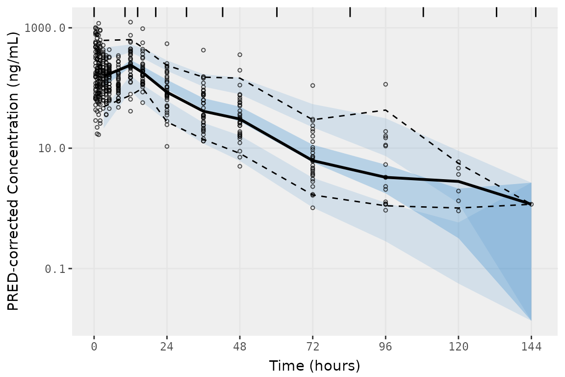
Whomp Whomp. bins = "density", like the previous methods
evaluated, grouped most of the absorption phase into a single bin.
##Exact bins in the input data
df_nobsbin(data_sad, bin_var = "NTIME")
#> # A tibble: 19 × 4
#>    NTIME   CMT n_obs n_miss
#>    <dbl> <dbl> <int>  <int>
#>  1   0       2     0     36
#>  2   0.5     2    34      2
#>  3   1       2    36      0
#>  4   1.5     2    36      0
#>  5   2       2    36      0
#>  6   3       2    36      0
#>  7   4       2    36      0
#>  8   5       2    36      0
#>  9   8       2    36      0
#> 10  12       2    36      0
#> 11  16       2    36      0
#> 12  24       2    36      0
#> 13  36       2    36      0
#> 14  48       2    33      3
#> 15  72       2    29      7
#> 16  96       2    16     20
#> 17 120       2     6     30
#> 18 144       2     1     35
#> 19 168       2     0     36

##Bin midpoints and boundaries determined by vpc() using bins = "density"
distinct(select(vpc_density$data, bin_mid, bin_min, bin_max))
#> Adding missing grouping variables: `strat`
#> # A tibble: 10 × 4
#> # Groups:   strat [1]
#>    strat bin_mid bin_min bin_max
#>    <fct>   <dbl>   <dbl>   <dbl>
#>  1 1        3.14     0      10.2
#>  2 1       12       10.2    14.4
#>  3 1       16       14.4    20.3
#>  4 1       24       20.3    30.4
#>  5 1       36       30.4    42.3
#>  6 1       48       42.3    60.2
#>  7 1       72       60.2    84.3
#>  8 1       96       84.3   108.
#>  9 1      120      108.    133.
#> 10 1      144      133.    145.
This leaves us with two methods that divide the data equally into
bins over the range of values in the data: bins = "data"
(equal data density in each bin) and bins = "time" (equal
bin width in time).
vpc_data <- vpc(
  sim = simout,
  obs = filter(simout, SIM == 1),
  bins = "data",
  sim_cols = list(dv = "SIMDV", idv = "NTIME", pred = "PRED"),
  obs_cols = list(dv = "OBSDV", idv = "NTIME", pred = "PRED"),
  pred_corr = TRUE,
  pi = c(0.05, 0.95),
  ci = c(0.05, 0.95),
  show = list(obs_dv = TRUE),
  log_y = TRUE,
  xlab = "Time (hours)",
  ylab = "PRED-corrected Concentration (ng/mL)"
) +
  scale_x_continuous(breaks = seq(0,168,24))

vpc_time <- vpc(
  sim = simout,
  obs = filter(simout, SIM == 1),
  bins = "time",
  sim_cols = list(dv = "SIMDV", idv = "NTIME", pred = "PRED"),
  obs_cols = list(dv = "OBSDV", idv = "NTIME", pred = "PRED"),
  pred_corr = TRUE,
  pi = c(0.05, 0.95),
  ci = c(0.05, 0.95),
  show = list(obs_dv = TRUE),
  log_y = TRUE,
  xlab = "Time (hours)",
  ylab = "PRED-corrected Concentration (ng/mL)"
) +
  scale_x_continuous(breaks = seq(0,168,24))

vpc_data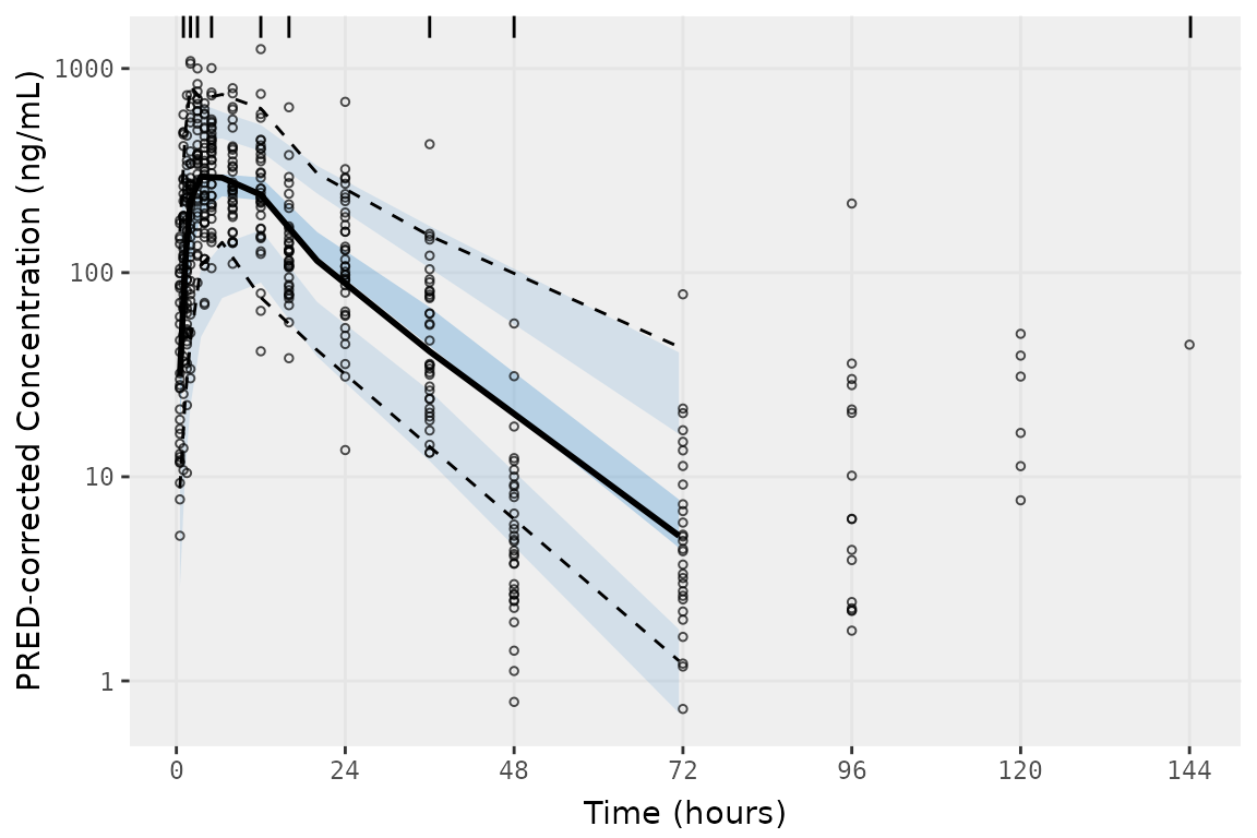
vpc_time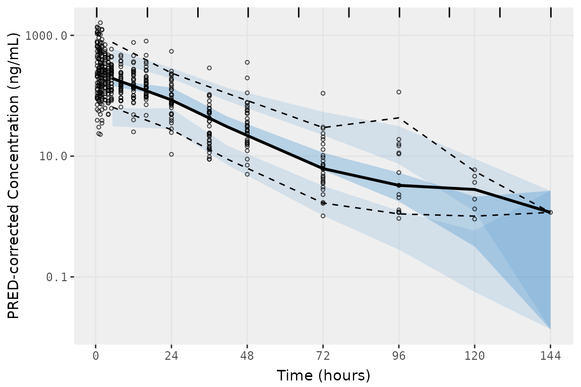
These methods are designed to equalize data density in each bin, which does not produce binning consistent with the exact bins in our dataset.
##Exact bins in the input data
df_nobsbin(data_sad, bin_var = "NTIME")
#> # A tibble: 19 × 4
#>    NTIME   CMT n_obs n_miss
#>    <dbl> <dbl> <int>  <int>
#>  1   0       2     0     36
#>  2   0.5     2    34      2
#>  3   1       2    36      0
#>  4   1.5     2    36      0
#>  5   2       2    36      0
#>  6   3       2    36      0
#>  7   4       2    36      0
#>  8   5       2    36      0
#>  9   8       2    36      0
#> 10  12       2    36      0
#> 11  16       2    36      0
#> 12  24       2    36      0
#> 13  36       2    36      0
#> 14  48       2    33      3
#> 15  72       2    29      7
#> 16  96       2    16     20
#> 17 120       2     6     30
#> 18 144       2     1     35
#> 19 168       2     0     36

##Bin midpoints and boundaries determined by vpc() using bins = "data"
distinct(select(vpc_data$data, bin_mid, bin_min, bin_max))
#> Adding missing grouping variables: `strat`
#> # A tibble: 9 × 4
#> # Groups:   strat [1]
#>   strat bin_mid bin_min bin_max
#>   <fct>   <dbl>   <dbl>   <dbl>
#> 1 1        1.25       1      2
#> 2 1        2          2      3
#> 3 1        3.5        3      5
#> 4 1        6.5        5     12
#> 5 1       12         12     16
#> 6 1       20         16     36
#> 7 1       36         36     48
#> 8 1       71.4       48    144.
#> 9 1        0.5       NA     NA

##Bin midpoints and boundaries determined by vpc() using bins = "time"
distinct(select(vpc_time$data, bin_mid, bin_min, bin_max))
#> Adding missing grouping variables: `strat`
#> # A tibble: 7 × 4
#> # Groups:   strat [1]
#>   strat bin_mid bin_min bin_max
#>   <fct>   <dbl>   <dbl>   <dbl>
#> 1 1        5.33   0.357    16.4
#> 2 1       24     16.4      32.4
#> 3 1       41.7   32.4      48.3
#> 4 1       72     64.3      80.2
#> 5 1       96     80.2      96.2
#> 6 1      120    112       128
#> 7 1      144    128       144.
VPC Plots with pmxhelpr
The pmxhelpr function plot_vpc_exactbins() is a wrapper
function for vpc(), which is optimized for input datasets
containing exact bins. This wrapper passes the the unique exact bins
(e.g., nominal times) in the input dataset as bin boundaries with the
addition of Inf to the end of the vector to ensure that the
final exact bin is included, rather than set only as a boundary.
This functionality can be reproduced using vpc() by
passing a vector of unique exact bins to bins with the
addition of Inf as follows:
bins = c(sort(unique(simout$NTIME)), Inf)
exact_bins <- c(sort(unique(simout$NTIME)), Inf)

vpc_exact_ntime <- vpc(
  sim = simout,
  obs = filter(simout, SIM == 1),
  bins = exact_bins,
  sim_cols = list(dv = "SIMDV", idv = "NTIME", pred = "PRED"),
  obs_cols = list(dv = "OBSDV", idv = "NTIME", pred = "PRED"),
  pred_corr = TRUE,
  pi = c(0.05, 0.95),
  ci = c(0.05, 0.95),
  show = list(obs_dv = TRUE),
  log_y = TRUE,
  xlab = "Time (hours)",
  ylab = "PRED-corrected Concentration (ng/mL)"
)+
  scale_x_continuous(breaks = seq(0,168,24))

vpc_exact_ntime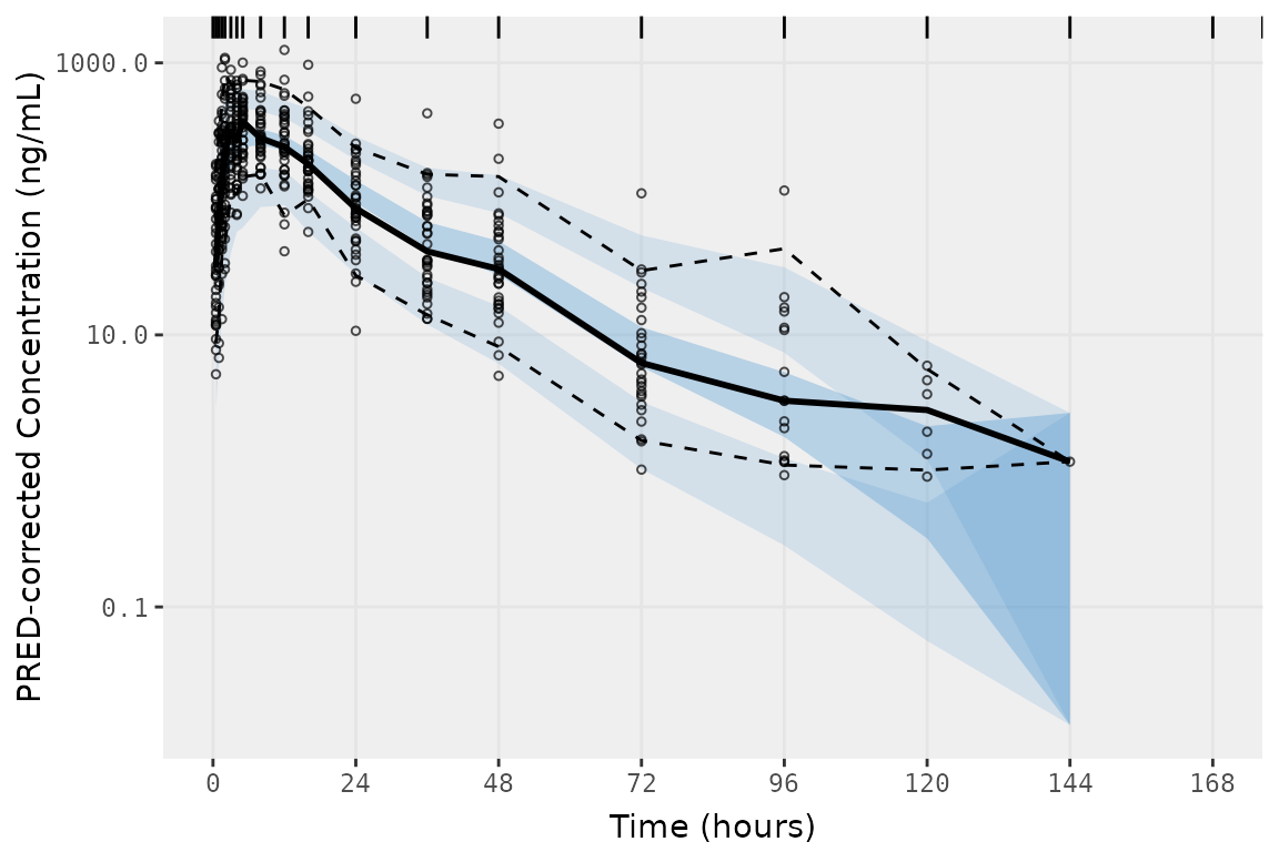
However, this workaround only works if idv is set to the
nominal time variable (idv = "NTIME) in both
sim_cols and obs_cols, which removes the
option to plot the observations by actual time
("TIME").
plot_vpc_exactbins() gets around this limitation by
plotting the observed data in a separate layer on top of the plot object
returned by vpc(), including prediction-correction of those
observed points if pcvpc = TRUE (also passed along to the
pred_corr argument of vpc()).
vpc_exact <- plot_vpc_exactbins(
  sim = simout,
  pcvpc = TRUE,
  time_vars = c(TIME = "TIME", NTIME = "NTIME"),
  output_vars = c(PRED = "PRED", IPRED = "IPRED", SIMDV = "SIMDV", OBSDV = "OBSDV"),
  pi = c(0.05, 0.95),
  ci = c(0.05, 0.95),
  xlab = "Time (hours)",
  ylab = "PRED-corrected Concentration (ng/mL)"
) +
  scale_y_log10(guide = "axis_logticks")

vpc_exact 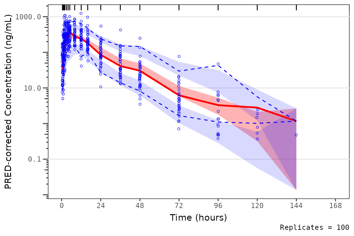
The difference in plotting the observed prediction-corrected data
points by "TIME" versus "NTIME" is negligible
for this example dataset, due to the high concordance between
"TIME" and "NTIME" in this example Phase 1
study. However, this difference is often much larger for pooled analyses
including later phase clinical studies where plotting the observed
points versus actual time will result in a plot that is much more
representative of the distribution of times in the model training
dataset.
When exploring the bins in the input and output datasets using
plot_vpc_exactbins(), we now see that they are consistent!
Huzzah!
##Exact bins in the input data
df_nobsbin(data_sad, bin_var = "NTIME")
#> # A tibble: 19 × 4
#>    NTIME   CMT n_obs n_miss
#>    <dbl> <dbl> <int>  <int>
#>  1   0       2     0     36
#>  2   0.5     2    34      2
#>  3   1       2    36      0
#>  4   1.5     2    36      0
#>  5   2       2    36      0
#>  6   3       2    36      0
#>  7   4       2    36      0
#>  8   5       2    36      0
#>  9   8       2    36      0
#> 10  12       2    36      0
#> 11  16       2    36      0
#> 12  24       2    36      0
#> 13  36       2    36      0
#> 14  48       2    33      3
#> 15  72       2    29      7
#> 16  96       2    16     20
#> 17 120       2     6     30
#> 18 144       2     1     35
#> 19 168       2     0     36

##Bin midpoints and boundaries determined by plot_vpc_exactbins()
distinct(select(vpc_exact$data, bin_mid, bin_min, bin_max))
#> Adding missing grouping variables: `strat`
#> # A tibble: 17 × 4
#> # Groups:   strat [1]
#>    strat bin_mid bin_min bin_max
#>    <fct>   <dbl>   <dbl>   <dbl>
#>  1 1         0.5     1       1.5
#>  2 1         1       1.5     2
#>  3 1         1.5     2       3
#>  4 1         2       3       4
#>  5 1         3       4       5
#>  6 1         4       5       8
#>  7 1         5       8      12
#>  8 1         8      12      16
#>  9 1        12      16      24
#> 10 1        16      24      36
#> 11 1        24      36       0.5
#> 12 1        36       0.5    48
#> 13 1        48      48      72
#> 14 1        72      72      96
#> 15 1        96      96     120
#> 16 1       120     120     144
#> 17 1       144     144     Inf
plot_vpc_exactbins() also contains an argument built
around df_nobsbin(). The argument
min_bin_count (default = 1) filters out exact bins with
fewer quantifiable observations than the minimum set by this argument.
Importantly, the observed data points in these small bins are still
plotted; however, they do not influence the calculation of summary
statistics or summary plot elements (shaded intervals, lines). This
provides the greatest fidelity to the data visualized without
introducing visual artifacts due to small sample timepoints.
Additionally, because our plot input dataset simout was
generated using df_mrgsim_replicate, the
time_vars and output_vars match the default
values, so we do not need to specify these arguments and they can be
removed. Furthermore, the pi and ci arguments
we are specifying match the default 90% PI and CI in vpc()
and can be removed.
When settingmin_bin_count = 10, summary statistics are
not plotted for the final two timepoint containing only fewer than 10
quantifiable observations; however, the observations themselves are
still plotted.
vpc_exact_bin_gt10 <- plot_vpc_exactbins(
  sim = simout,
  pcvpc = TRUE,
  min_bin_count = 10,
  xlab = "Time (hours)",
  ylab = "PRED-corrected Concentration (ng/mL)"
) +
  scale_y_log10(guide = "axis_logticks")

vpc_exact_bin_gt10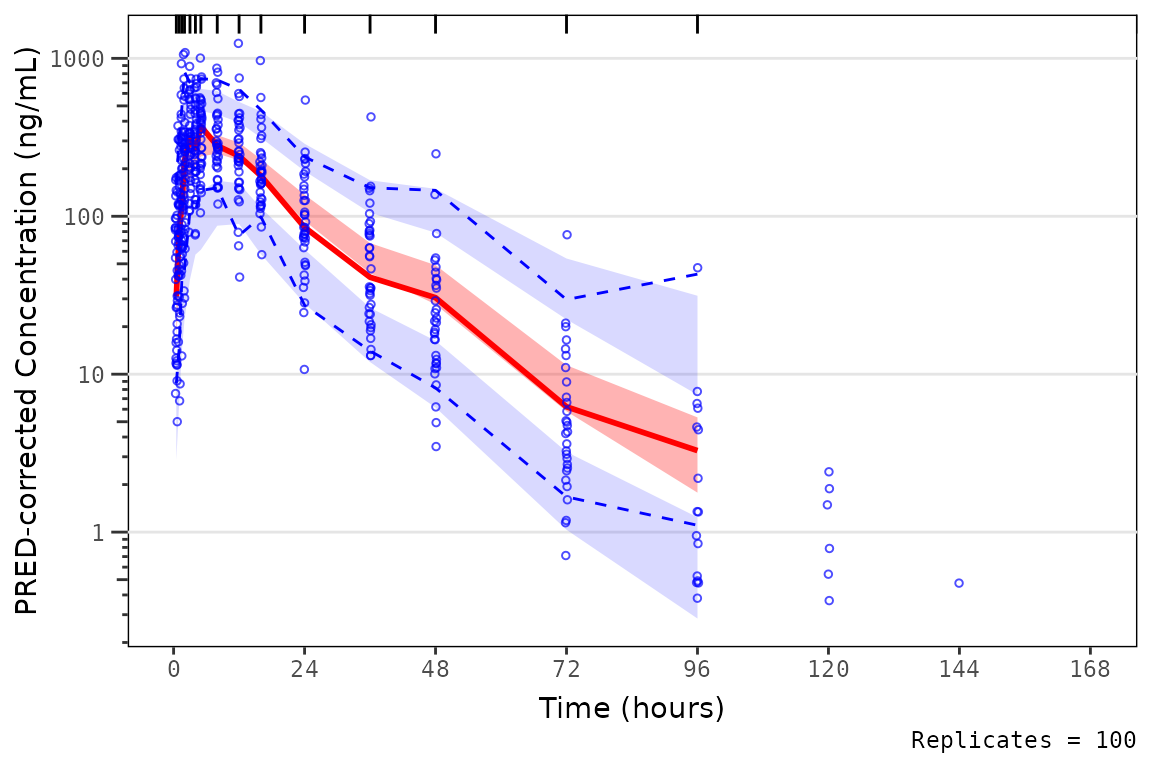
We can also pass stratifying variables to the argument
strat_var in order to facet our plots by relevant covariate
conditions. The stratification variables specified in
strat_var are also passed to the stratify
argument of vpc(), in order to facet the resulting plots.
Currently, only one variable can be passed to this argument.
vpc_exact_food <- plot_vpc_exactbins(
  sim = mutate(simout, FOOD_f = factor(FOOD, levels = c(0,1), labels = c("Fasted", "Fed"))),
  strat_var = "FOOD_f",
  pcvpc = TRUE,
  xlab = "Time (hours)",
  ylab = "PRED-corrected Concentration (ng/mL)",
  min_bin_count = 4
) +
  scale_y_log10(guide = "axis_logticks")

vpc_exact_food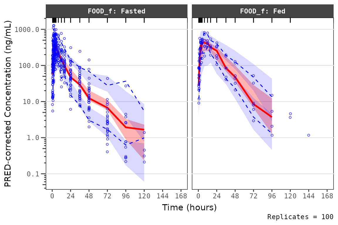
Note that all these plots add a layer to the ggplot2
object returned by plot_vpc_exactbins to transform the
y-axis from linear to log10 scales. One could specify the
log_y argument in plot_vpc_exactbins, which is
not native to plot_vpc_exactbins, but will be passed to
vpc::vpc.
It is important to understand how the data are handled within
vpc::vpc() when specifying the log_y argument.
From the vpc::vpc() function documentation:
-
log_y: Boolean indicting whether y-axis should be shown as logarithmic. Default is FALSE. -
log_y_min: minimal value when using log_y argument. Default is 1e-3.
Therefore, vpc::vpc() will will transform the data prior
to calculating summary statistics and plotting by imputing any values
< log_y_min to the value specified in this argument
(default = 0.001). Therefore, if there are observed values less than
this threshold, they will be censored at this minimum.
This can lead to unexpected behavior if data fall in a very low
concentration range and the log_y_min argument is not
specified.
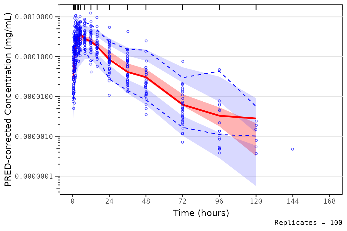
vpc_exact_transform_logy <- plot_vpc_exactbins(
  sim = mutate(simout,
               PRED = PRED/(10^6),
               OBSDV = OBSDV/(10^6),
               SIMDV = SIMDV/(10^6)),
  pcvpc = TRUE,
  xlab = "Time (hours)",
  ylab = "PRED-corrected Concentration (mg/mL)",
  min_bin_count = 4,
  log_y = TRUE
)

vpc_exact_transform_logy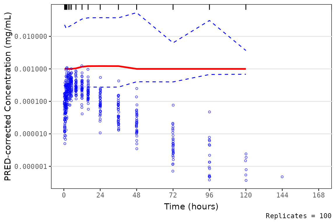
Thus, to avoid unexpected censoring of data on the VPC plot, one can
plot without specifying log_y and then add a new log10
scale for the y-axis.
vpc_exact_transform_yscale <- plot_vpc_exactbins(
  sim = mutate(simout,
               PRED = PRED/(10^6),
               OBSDV = OBSDV/(10^6),
               SIMDV = SIMDV/(10^6)),
  pcvpc = TRUE,
  xlab = "Time (hours)",
  ylab = "PRED-corrected Concentration (mg/mL)",
  min_bin_count = 4
)  +
  scale_y_log10(guide = "axis_logticks")

vpc_exact_transform_yscale